NASA dataset keywords analysis: Neo4j analytics tutorial

In this notebook we use graph-based co-occurrence analysis on the publicly available Data catalog of NASA (https://data.nasa.gov/browse, and the API endpoint https://data.nasa.gov/data.json). This dataset consists of the meta-data for different NASA datasets. The source notebook can be found here.

We will work on the sets of keywords attached to each dataset and build a keyword co-occurrence graph describing relations between different dataset keywords. The keyword relations in the above-mentioned graph are quantified using mutual-information-based scores (normalized pointwise mutual information).

See the related tutorial here: https://www.tidytextmining.com/nasa.html

In this tutorial we will use the Neo4j-based implementation of different analytics interfaces provided by BlueGraph. Therefore, in order to use it, you need a running instance of the Neo4j database (see installation instructions).

import os
import json
import pandas as pd
import requests
import getpass

from bluegraph.core import (PandasPGFrame,
                            pretty_print_paths,
                            pretty_print_tripaths)
from bluegraph.preprocess.generators import CooccurrenceGenerator
from bluegraph.backends.neo4j import (pgframe_to_neo4j,
                                      Neo4jMetricProcessor,
                                      Neo4jPathFinder,
                                      Neo4jCommunityDetector,
                                      Neo4jGraphProcessor)
from bluegraph.backends.networkx import NXPathFinder, networkx_to_pgframe

Data preparation

Download and read the NASA dataset.

NASA_META_DATA_URL = "https://data.nasa.gov/data.json"
if not os.path.isfile("../data/nasa.json"):
    r = requests.get(NASA_META_DATA_URL)
    open("../data/nasa.json", "wb").write(r.content)

with open("../data/nasa.json", "r") as f:
    data = json.load(f)

print("Example dataset: ")
print("----------------")
print(json.dumps(data["dataset"][0], indent="   "))

print()
print("Keywords: ", data["dataset"][0]["keyword"])

Example dataset:
----------------
{
   "accessLevel": "public",
   "landingPage": "https://pds.nasa.gov/ds-view/pds/viewDataset.jsp?dsid=RO-E-RPCMAG-2-EAR2-RAW-V3.0",
   "bureauCode": [
      "026:00"
   ],
   "issued": "2018-06-26",
   "@type": "dcat:Dataset",
   "modified": "2020-03-04",
   "references": [
      "https://pds.nasa.gov"
   ],
   "keyword": [
      "earth",
      "unknown",
      "international rosetta mission"
   ],
   "contactPoint": {
      "@type": "vcard:Contact",
      "fn": "Thomas Morgan",
      "hasEmail": "mailto:thomas.h.morgan@nasa.gov"
   },
   "publisher": {
      "@type": "org:Organization",
      "name": "National Aeronautics and Space Administration"
   },
   "identifier": "urn:nasa:pds:context_pds3:data_set:data_set.ro-e-rpcmag-2-ear2-raw-v3.0",
   "description": "This dataset contains EDITED RAW DATA of the second Earth Flyby (EAR2). The closest approach (CA) took place on November 13, 2007 at 20:57",
   "title": "ROSETTA-ORBITER EARTH RPCMAG 2 EAR2 RAW V3.0",
   "programCode": [
      "026:005"
   ],
   "distribution": [
      {
         "@type": "dcat:Distribution",
         "downloadURL": "https://www.socrata.com",
         "mediaType": "text/html"
      }
   ],
   "accrualPeriodicity": "irregular",
   "theme": [
      "Earth Science"
   ]
}

Keywords:  ['earth', 'unknown', 'international rosetta mission']

Create a dataframe with keyword occurrence in different datasets

rows = []
for el in data['dataset']:
    row = [el["identifier"]]
    if "keyword" in el:
        for k in el["keyword"]:
            rows.append(row + [k])
keyword_data = pd.DataFrame(rows, columns=["dataset", "keyword"])

keyword_data

	dataset	keyword
0	urn:nasa:pds:context_pds3:data_set:data_set.ro...	earth
1	urn:nasa:pds:context_pds3:data_set:data_set.ro...	unknown
2	urn:nasa:pds:context_pds3:data_set:data_set.ro...	international rosetta mission
3	TECHPORT_9532	completed
4	TECHPORT_9532	jet propulsion laboratory
...	...	...
112731	NASA-877__2	lunar
112732	NASA-877__2	jsc
112733	NASA-877__2	sample
112734	TECHPORT_94299	active
112735	TECHPORT_94299	trustees of the colorado school of mines

112736 rows × 2 columns

Aggregate dataset ids for each keyword and select the 500 most frequently used keywords.

n = 500

aggregated_datasets = keyword_data.groupby("keyword").aggregate(set)["dataset"]
most_frequent_keywords = list(aggregated_datasets.apply(len).nlargest(n).index)
most_frequent_keywords[:5]

['completed',
 'earth science',
 'atmosphere',
 'national geospatial data asset',
 'ngda']

Create a property graph object whose nodes are unique keywords.

graph = PandasPGFrame()
graph.add_nodes(most_frequent_keywords)
graph.add_node_types({n: "Keyword" for n in most_frequent_keywords})

Add sets of dataset ids as properties of our keyword nodes.

aggregated_datasets.index.name = "@id"
graph.add_node_properties(aggregated_datasets, prop_type="category")

graph._nodes.sample(5)

	@type	dataset
@id
4 vesta	Keyword	{urn:nasa:pds:context_pds3:data_set:data_set.d...
jsc	Keyword	{NASA-872, NASA-877, NASA-873, NASA-871, NASA-...
paaliaq	Keyword	{urn:nasa:pds:context_pds3:data_set:data_set.c...
international halley watch	Keyword	{urn:nasa:pds:context_pds3:data_set:data_set.i...
active remote sensing	Keyword	{C1243149604-ASF, C1243162394-ASF, C1243197502...

n_datasets = len(keyword_data["dataset"].unique())
print("Total number of dataset: ", n_datasets)

Total number of dataset:  25722

Co-occurrence graph generation

We create a co-occurrence graph using the 500 most frequent keywords: nodes are keywords and a pair of nodes is connected with an undirected edge if two corresponding keywords co-occur in at lease one dataset. Moreover, the edges are equipped with weights corresponding to:

• raw co-occurrence frequency

• normalized pointwise mutual information (NPMI)

• frequency- and mutual-information-based distances (1 / frequency, 1 / NPMI)

generator = CooccurrenceGenerator(graph)
comention_edges = generator.generate_from_nodes(
    "dataset", total_factor_instances=n_datasets,
    compute_statistics=["frequency", "npmi"])

Examining 124750 pairs of terms for co-occurrence...

Remove edges with zero NPMI

comention_edges = comention_edges[comention_edges["npmi"] > 0]

Compute the NPMI-based distance score

comention_edges.loc[:, "distance_npmi"] = comention_edges.loc[:, "npmi"].apply(lambda x: 1 / x)

Add generated edges to the property graph.

graph.remove_node_properties("dataset") # Remove datasets from node properties
graph._edges = comention_edges.drop(columns=["common_factors"])
graph._edge_prop_types = {
    "frequency": "numeric",
    "npmi": "numeric",
    "distance_npmi": "numeric"
}

graph.edges(raw_frame=True).sample(5)

		frequency	npmi	distance_npmi
@source_id	@target_id
surface radiative properties	natural hazards	3	0.022294	44.855423
cryosphere	radar	56	0.248405	4.025688
mars global surveyor	stardust	2	0.395268	2.529931
sample treatment protocol	temperature	1	0.446902	2.237629
radar	synthetic	1	0.056982	17.549306

Initializing Neo4j graph from a PGFrame

In this section we will populate a Neo4j database with the generated keyword co-occurrence property graph.

In the cells below provide the credentials for connecting to your instance of the Neo4j database.

NEO4J_URI = "bolt://localhost:7687"
NEO4J_USER = "neo4j"

NEO4J_PASSWORD = getpass.getpass()

········

Populate the Neo4j database with the nodes and edges of the generated property graph using pgframe_to_neo4j. We specify labels of nodes (Keyword) and edges (CoOccurs) to use for the new elements.

NODE_LABEL = "Keyword"
EDGE_LABEL = "CoOccurs"

# (!) If you run this cell multiple times, you may create nodes and edges of the graph
# multiple times, if you have already run the notebook, set the parameter `pgframe` to None
# this will prevent population of the Neo4j database with the generated graph, but will create
# the necessary `Neo4jGraphView` object.
graph_view = pgframe_to_neo4j(
    pgframe=graph,  # None, if no population is required
    uri=NEO4J_URI, username=NEO4J_USER, password=NEO4J_PASSWORD,
    node_label=NODE_LABEL, edge_label=EDGE_LABEL,
    directed=False)

# # If you want to clear the database from created elements, run
# graph_view._clear()

Nearest neighours by NPMI

In this section we will compute top 10 neighbors of the keywords ‘mars’ and ‘saturn’ by the highest NPMI.

To do so, we will use the top_neighbors method of the PathFinder interface provided by the BlueGraph. This interface allows us to search for top neighbors with the highest edge weight. In this example, we use Neo4j-based Neo4jPathFinder interface.

path_finder = Neo4jPathFinder.from_graph_object(graph_view)

path_finder.top_neighbors("mars", 10, weight="npmi")

{'mars exploration rover': 0.7734334910676389,
 'phoenix': 0.6468063979421724,
 'mars science laboratory': 0.6354738555723674,
 '2001 mars odyssey': 0.5902693119742288,
 'mars global surveyor': 0.5756873488729959,
 'mars reconnaissance orbiter': 0.555421194053889,
 'viking': 0.5490894121185264,
 'mars pathfinder': 0.5223639673427369,
 'mars express': 0.5153112375202485,
 'phobos': 0.49283414887183974}

path_finder.top_neighbors("saturn", 10, weight="npmi")

{'iapetus': 0.7512958866945076,
 'tethys': 0.750629376973449,
 'mimas': 0.7481024499128304,
 'phoebe': 0.7458314316016054,
 'rhea': 0.7453385116030462,
 'dione': 0.7425859139664013,
 'cassini-huygens': 0.74217432172955,
 'enceladus': 0.7347323196182364,
 'hyperion': 0.7346061630878281,
 'janus': 0.7144193057581066}

Graph metrics and node centrality measures

BlueGraph provides the MetricProcessor interface for computing various graph statistics. We will use Neo4j-based Neo4jMetricProcessor interface.

metrics = Neo4jMetricProcessor.from_graph_object(graph_view)

print("Density of the constructed network: ", metrics.density())

Density of the constructed network:  0.051334669338677356

Node centralities

In this example we will compute the Degree and PageRank centralities only for the raw frequency, and the Betweenness centrality for the mutual-information-based scores. We will use methods provided by the MetricProcessor interface in the write mode, i.e. computed metrics will be written as node properties of the underlying graph object.

Degree centrality is given by the sum of weights of all incident edges of the given node and characterizes the importance of the node in the network in terms of its connectivity to other nodes (high degree = high connectivity).

metrics.degree_centrality("frequency", write=True, write_property="degree")

PageRank centrality is another measure that estimated the importance of the given node in the network. Roughly speaking it can be interpreted as the probablity that having landed on a random node in the network we will jump to the given node (here the edge weights are taken into account”).

https://en.wikipedia.org/wiki/PageRank

metrics.pagerank_centrality("frequency", write=True, write_property="pagerank")

We then compute the betweenness centrality based on the NPMI distances.

Betweenness centrality is a node importance measure that estimates how often a shortest path between a pair of nodes will pass through the given node.

metrics.betweenness_centrality("distance_npmi", write=True, write_property="betweenness")

/Users/oshurko/opt/anaconda3/envs/bluegraph/lib/python3.6/site-packages/bluegraph/backends/neo4j/analyse/metrics.py:111: MetricProcessingWarning: Weighted betweenness centrality for Neo4j graphs is not implemented: computing the unweighted version
  MetricProcessor.MetricProcessingWarning)

Now, we will export this backend-specific graph object into a PGFrame.

new_graph = metrics.get_pgframe(node_prop_types=graph._node_prop_types, edge_prop_types=graph._edge_prop_types)

new_graph.nodes(raw_frame=True).sample(5)

	degree	betweenness	pagerank
@id
delta	25.0	122.525847	0.948799
langley research center	2.0	2.832536	0.553508
radiation dosimetry	33.0	60.795710	1.255296
population	25.0	49.157125	0.729864
tarvos	32.0	0.000000	0.923662

print("Top 10 nodes by degree")
for n in new_graph.nodes(raw_frame=True).nlargest(10, columns=["degree"]).index:
    print("\t", n)

Top 10 nodes by degree
     earth science
     jupiter
     earth
     land surface
     terrestrial hydrosphere
     imagery
     support archives
     sun
     atmosphere
     surface water

print("Top 10 nodes by PageRank")
for n in new_graph.nodes(raw_frame=True).nlargest(10, columns=["pagerank"]).index:
    print("\t", n)

Top 10 nodes by PageRank
     active
     earth science
     completed
     project
     pds
     earth
     jupiter
     imagery
     data
     moon

print("Top 10 nodes by betweenness")
for n in new_graph.nodes(raw_frame=True).nlargest(10, columns=["betweenness"]).index:
    print("\t", n)

Top 10 nodes by betweenness
     astronomy
     imagery
     goddard space flight center
     radar
     active
     topography
     safety
     time
     images
     temperature

Community detection

Community detection methods partition the graph into clusters of densely connected nodes in a way that nodes in the same community are more connected between themselves relatively to the nodes in different communities. In this section we will illustrate the use of the CommunityDetector interface provided by BlueGraph for community detection and estimation of its quality using modularity, performance and coverange methods.

First, we create a Neo4j-based instance and use several different community detection strategies provided by Neo4j.

com_detector = Neo4jCommunityDetector.from_graph_object(graph_view)

Louvain algorithm

partition = com_detector.detect_communities(
    strategy="louvain", weight="npmi")

print("Modularity: ", com_detector.evaluate_parition(partition, metric="modularity", weight="npmi"))
print("Performance: ", com_detector.evaluate_parition(partition, metric="performance", weight="npmi"))
print("Coverage: ", com_detector.evaluate_parition(partition, metric="coverage", weight="npmi"))

Modularity:  0.8055352122880087
Performance:  0.9050420841683366
Coverage:  0.9223953224304512

Label propagation

partition = com_detector.detect_communities(
    strategy="lpa", weight="npmi")

print("Modularity: ", com_detector.evaluate_parition(partition, metric="modularity", weight="npmi"))
print("Performance: ", com_detector.evaluate_parition(partition, metric="performance", weight="npmi"))
print("Coverage: ", com_detector.evaluate_parition(partition, metric="coverage", weight="npmi"))

Modularity:  0.6599097374293331
Performance:  0.6372184368737475
Coverage:  0.9699235341510681

Writing community partition as node properties

com_detector.detect_communities(
    strategy="louvain", weight="npmi",
    write=True, write_property="louvain_community")

new_graph = com_detector.get_pgframe(
    node_prop_types=new_graph._node_prop_types,
    edge_prop_types=new_graph._edge_prop_types)

new_graph.nodes(raw_frame=True).sample(5)

	degree	betweenness	louvain_community	pagerank
@id
sample collection	29.0	251.402898	330	1.130440
atmospheric chemistry	50.0	134.337209	319	1.304748
neptune	48.0	2524.723644	353	1.602773
coanda	8.0	0.000000	141	0.696748
phobos	49.0	868.444670	353	1.426603

Export network and the computed metrics

Save graph as JSON

new_graph.export_json("../data/nasa_comention.json")

Save the graph for Gephi import.

new_graph.export_to_gephi(
    "../data/gephi_nasa_comention",
    node_attr_mapping = {
        "degree": "Degree",
        "pagerank": "PageRank",
        "betweenness": "Betweenness",
        "louvain_community": "Community"
    },
    edge_attr_mapping={
        "npmi": "Weight"
    })

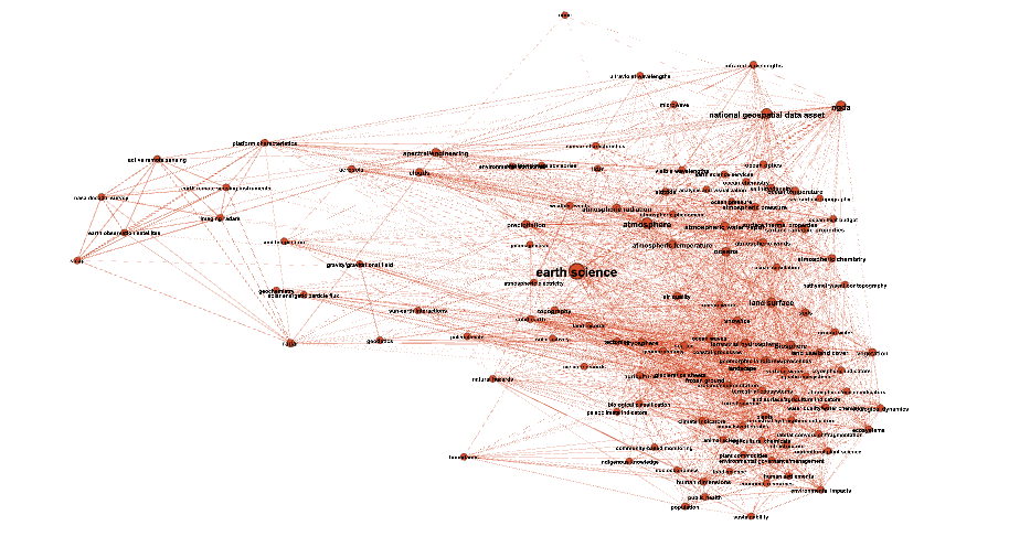
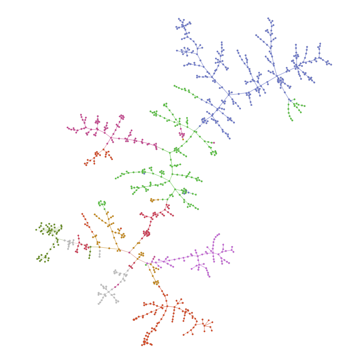
The representation of the network saved above can be imported into Gephi for producing graph visualizations, as in the following example:

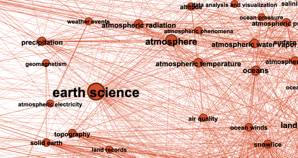
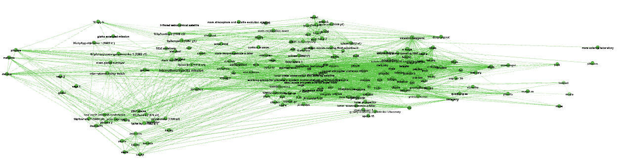
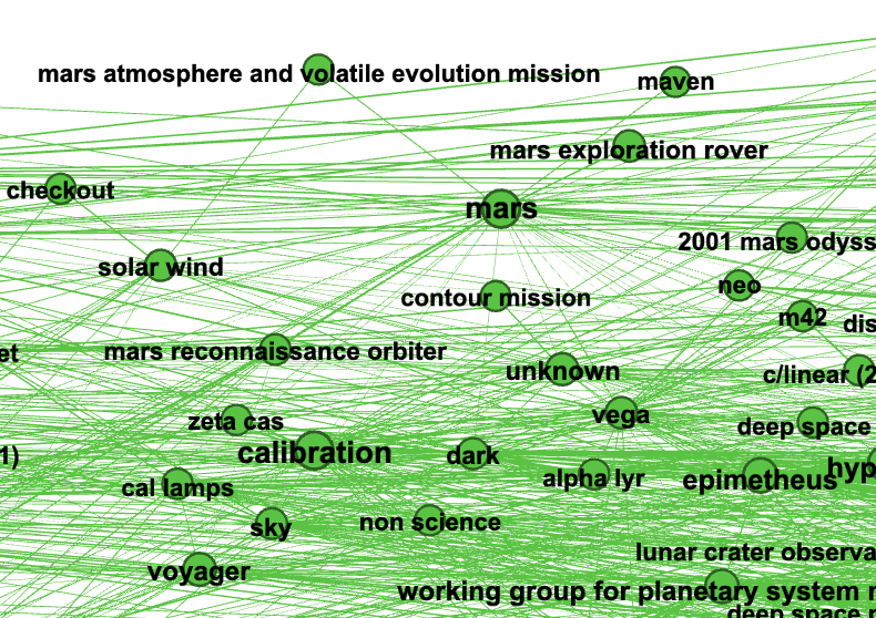
In the figures below colors represent communities detected using the raw frequency of the co-occurrence edges, node sizes are proportional to the PageRank of nodes and edge thickness to the NPMI values.

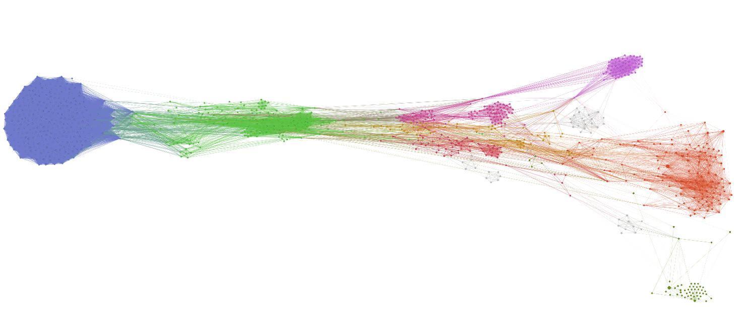
We can zoom into some of the communities of keywords identified using the community detection method above

Celestial bodies

Earth science

Space programs and missions

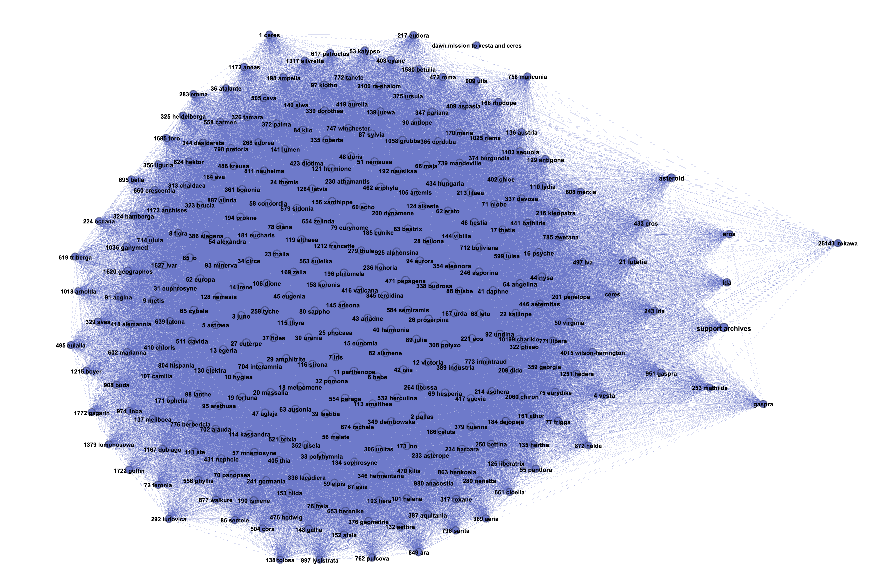
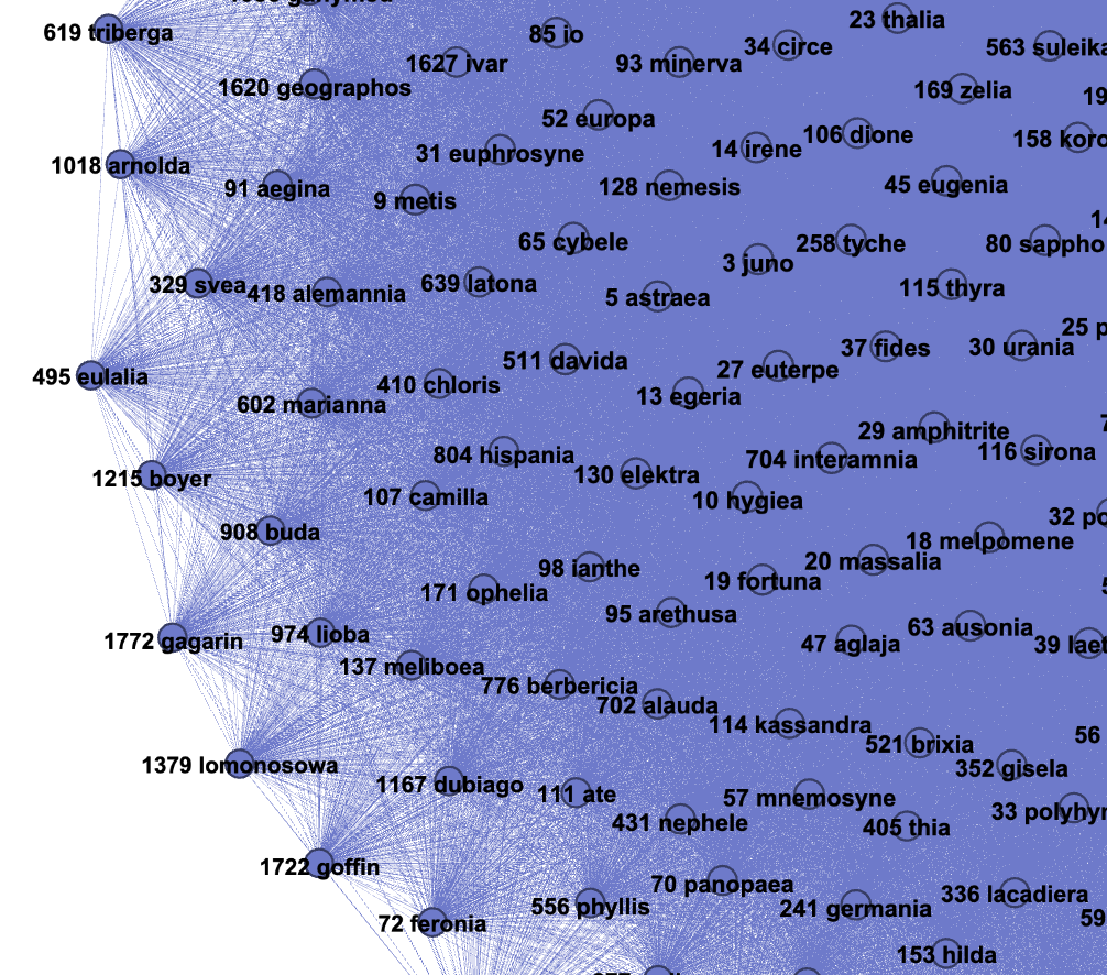
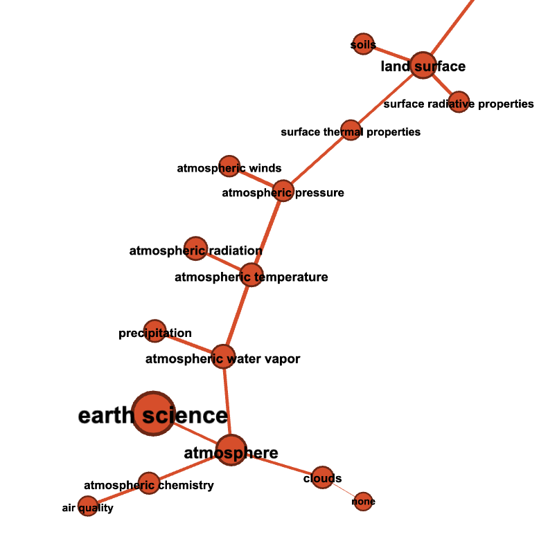
Minimum spanning tree

A minimum spanning tree of a network is given by a subset of edges that make the network connected (\(n - 1\) edges connecting \(n\) nodes). Its weighted version minimizes not only the number of edges included in the tree, but the total edge weight.

In the following example we compute a minimum spanning tree minimizing the NPMI-based distance weight of the network edges. We use the Neo4j-based implementation of the PathFinder interface.

path_finder.minimum_spanning_tree(distance="distance_npmi", write=True, write_edge_label="MSTEdge")

nx_path_finder = NXPathFinder(new_graph, directed=False)
tree = nx_path_finder.minimum_spanning_tree(distance="distance_npmi")

tree_pgframe = networkx_to_pgframe(
    tree,
    node_prop_types=new_graph._node_prop_types,
    edge_prop_types=new_graph._edge_prop_types)

tree_pgframe.export_to_gephi(
    "../data/gephi_nasa_spanning_tree",
    node_attr_mapping = {
        "degree": "Degree",
        "pagerank": "PageRank",
        "betweenness": "Betweenness",
        "louvain_community": "Community"
    },
    edge_attr_mapping={
        "npmi": "Weight"
    })

Zoom Earth Science

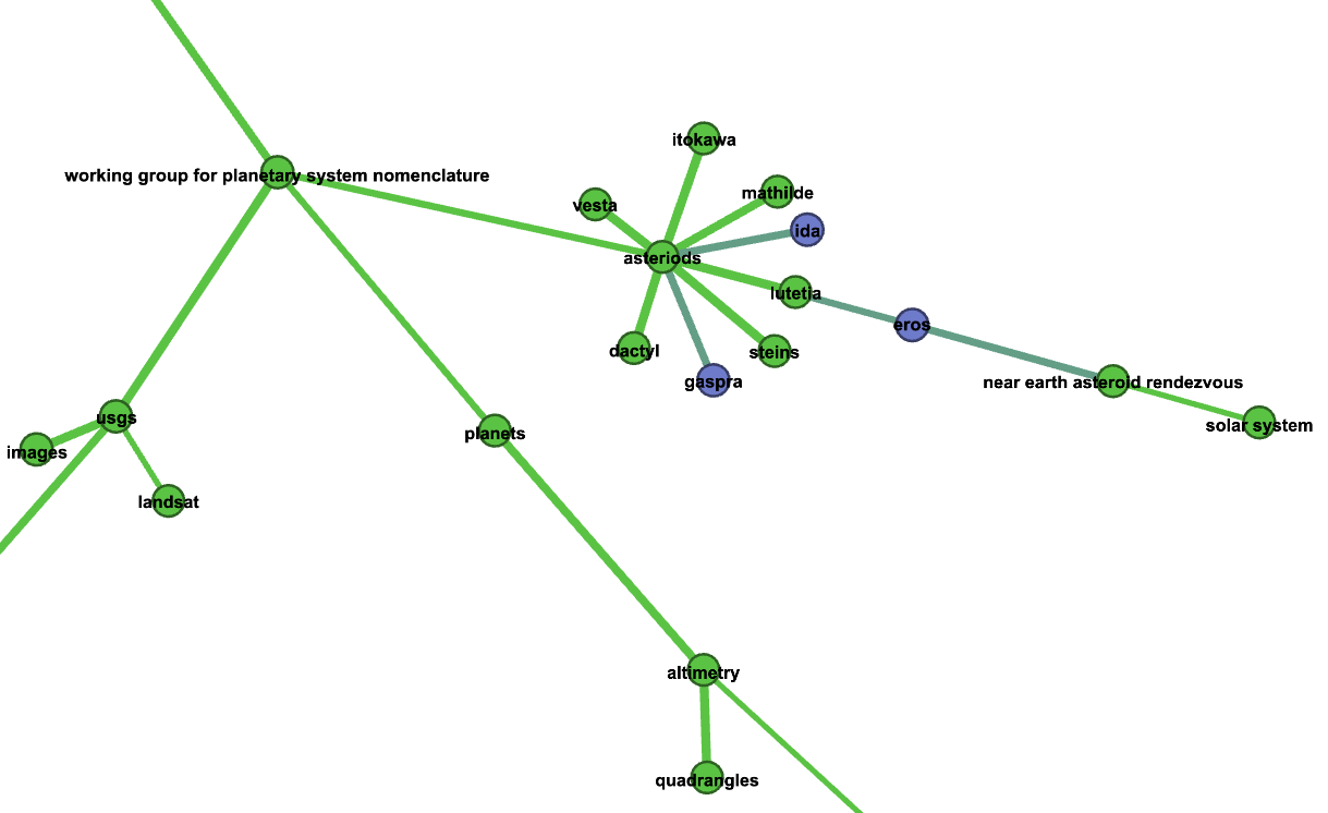
Zoom Asteroids

Shortest path search

The shortest path search problem consisits in finding a sequence of edges from the source node to the target node that minimizes the cumulative weight (or distance) associated to the edges.

path = path_finder.shortest_path("ecosystems", "oceans")
pretty_print_paths([path])

ecosystems <->               <-> oceans
               earth science

The cell above illustrates that the single shortest path form ‘ecosystems’ and ‘oceans’ consists of the direct edge between them.

Now to explore related keywords we would like to find a set of \(n\) shortest paths between them. Moreover, we would like these paths to be indirect (not to include the direct edge from the source to the target). In the following examples we use mutual-information-based edge weights to perform our literature exploration.

In the following examples we use Yen’s algorithm for finding \(n\) loopless shortest paths from the source to the target (https://en.wikipedia.org/wiki/Yen%27s_algorithm).

paths = path_finder.n_shortest_paths(
    "ecosystems", "oceans", n=10,
    distance="distance_npmi",
    strategy="yen")

pretty_print_paths(paths)

ecosystems <->                                              <-> oceans
               biosphere <-> coastal processes
               biosphere <-> ocean waves
               biosphere <-> terrestrial ecosystems
               biosphere <-> erosion/sedimentation
               geomorphic landforms/processes
               biosphere <-> geomorphic landforms/processes
               land use/land cover <-> coastal processes
               biosphere <-> forest science
               earth science
               land use/land cover <-> ocean waves

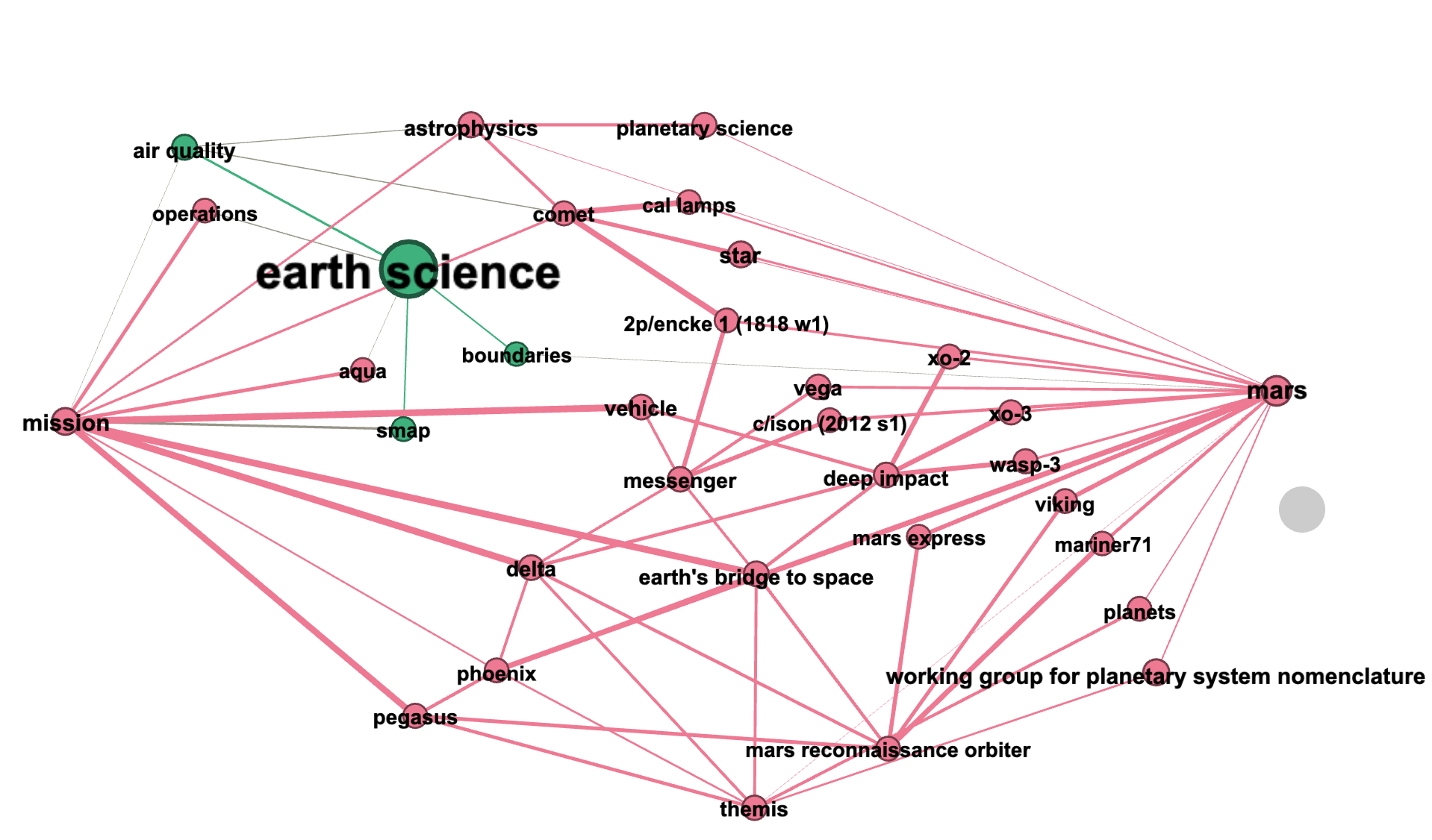
paths = path_finder.n_shortest_paths(
    "mission", "mars", n=10,
    distance="distance_npmi",
    strategy="yen")

pretty_print_paths(paths)

mission <->                                                         <-> mars
            delta <-> mars reconnaissance orbiter
            earth's bridge to space <-> mars reconnaissance orbiter
            vehicle <-> mars reconnaissance orbiter
            mars reconnaissance orbiter
            history <-> mars reconnaissance orbiter
            support <-> mars reconnaissance orbiter
            landing <-> mars reconnaissance orbiter
            delta <-> phoenix
            earth's bridge to space <-> phoenix
            vehicle <-> phoenix

Nested path search

To explore the space of co-occurring terms in depth, we can run the path search procedure presented above in a nested fashion. For each edge \(e_1, e_2, ..., e_n\) encountered on a path from the source to the target from, we can further expand it into \(n\) shortest paths between each pair of successive entities (i.e. paths between \(e_1\) and \(e_2\), \(e_2\) and \(e_3\), etc.).

paths1 = path_finder.n_nested_shortest_paths(
    "ecosystems", "oceans",
    top_level_n=10, nested_n=3, depth=2, distance="distance_npmi",
    strategy="yen")

paths2 = path_finder.n_nested_shortest_paths(
    "mission", "mars",
    top_level_n=10, nested_n=3, depth=2, distance="distance_npmi",
    strategy="yen")

We can now build and visualize the subnetwork constructed using the nodes and the edges discovered during our nested path search.

summary_graph_oceans = networkx_to_pgframe(nx_path_finder.get_subgraph_from_paths(paths1))
summary_graph_mars = networkx_to_pgframe(nx_path_finder.get_subgraph_from_paths(paths2))

# Save the graph for Gephi import.
summary_graph_oceans.export_to_gephi(
    "../data/gephi_nasa_path_graph_oceans",
    node_attr_mapping = {
        "degree": "Degree",
        "pagerank": "PageRank",
        "betweenness": "Betweenness",
        "louvain_community": "Community"
    },
    edge_attr_mapping={
        "npmi": "Weight"
    })
# Save the graph for Gephi import.
summary_graph_mars.export_to_gephi(
    "../data/gephi_nasa_path_graph_mars",
    node_attr_mapping = {
        "degree": "Degree",
        "pagerank": "PageRank",
        "betweenness": "Betweenness",
        "louvain_community": "Community"
    },
    edge_attr_mapping={
        "npmi": "Weight"
    })

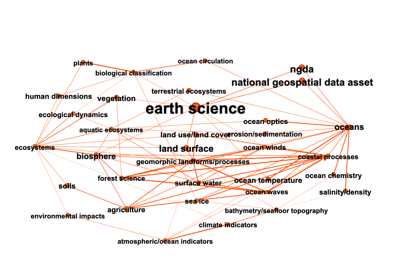
The resulting graphs visualized with Gephi

Ecosystems <-> Oceans

Mission <-> Mars