Embedding and downstream tasks tutorial
This tutorial illustrates an example of a co-occurrence graph and guides the user through the graph representation learning and all it’s downstream tasks including node similarity queries, node classification, edge prediction and embedding pipeline building. The source notebook can be found here.
import pandas as pd
import numpy as np

from sklearn import model_selection
from sklearn import mixture
from sklearn.svm import LinearSVC
from bluegraph.core import PandasPGFrame
from bluegraph.preprocess.generators import CooccurrenceGenerator
from bluegraph.preprocess.encoders import ScikitLearnPGEncoder

from bluegraph.core.embed.embedders import GraphElementEmbedder
from bluegraph.backends.stellargraph import StellarGraphNodeEmbedder

from bluegraph.downstream import EmbeddingPipeline, transform_to_2d, plot_2d, get_classification_scores
from bluegraph.downstream.similarity import (FaissSimilarityIndex,
                                             SimilarityProcessor,
                                             NodeSimilarityProcessor)
from bluegraph.downstream.node_classification import NodeClassifier
from bluegraph.downstream.link_prediction import (generate_negative_edges,
                                                  EdgePredictor)
Data preparation
Fist, we read the source dataset with mentions of entities in different paragraphs
mentions = pd.read_csv("../data/labeled_entity_occurrence.csv")
# Extract unique paper/seciton/paragraph identifiers
mentions = mentions.rename(columns={"occurrence": "paragraph"})
number_of_paragraphs = len(mentions["paragraph"].unique())
mentions
| entity | paragraph | |
|---|---|---|
| 0 | lithostathine-1-alpha | 1 |
| 1 | pulmonary | 1 |
| 2 | host | 1 |
| 3 | lithostathine-1-alpha | 2 |
| 4 | surfactant protein d measurement | 2 |
| ... | ... | ... |
| 2281346 | covid-19 | 227822 |
| 2281347 | covid-19 | 227822 |
| 2281348 | viral infection | 227823 |
| 2281349 | lipid | 227823 |
| 2281350 | inflammation | 227823 |
2281351 rows × 2 columns
We will also load a dataset that contains definitions of entities and their types
entity_data = pd.read_csv("../data/entity_types_defs.csv")
entity_data
| entity | entity_type | definition | |
|---|---|---|---|
| 0 | (e3-independent) e2 ubiquitin-conjugating enzyme | PROTEIN | (E3-independent) E2 ubiquitin-conjugating enzy... |
| 1 | (h115d)vhl35 peptide | CHEMICAL | A peptide vaccine derived from the von Hippel-... |
| 2 | 1,1-dimethylhydrazine | DRUG | A clear, colorless, flammable, hygroscopic liq... |
| 3 | 1,2-dimethylhydrazine | CHEMICAL | A compound used experimentally to induce tumor... |
| 4 | 1,25-dihydroxyvitamin d(3) 24-hydroxylase, mit... | PROTEIN | 1,25-dihydroxyvitamin D(3) 24-hydroxylase, mit... |
| ... | ... | ... | ... |
| 28127 | zygomycosis | DISEASE | Any infection due to a fungus of the Zygomycot... |
| 28128 | zygomycota | ORGANISM | A phylum of fungi that are characterized by ve... |
| 28129 | zygosity | ORGANISM | The genetic condition of a zygote, especially ... |
| 28130 | zygote | CELL_COMPARTMENT | The cell formed by the union of two gametes, e... |
| 28131 | zyxin | ORGANISM | Zyxin (572 aa, ~61 kDa) is encoded by the huma... |
28132 rows × 3 columns
Generation of a co-occurrence graph
We first create a graph whose nodes are entities
graph = PandasPGFrame()
entity_nodes = mentions["entity"].unique()
graph.add_nodes(entity_nodes)
graph.add_node_types({n: "Entity" for n in entity_nodes})

entity_props = entity_data.rename(columns={"entity": "@id"}).set_index("@id")
graph.add_node_properties(entity_props["entity_type"], prop_type="category")
graph.add_node_properties(entity_props["definition"], prop_type="text")
paragraph_prop = pd.DataFrame({"paragraphs": mentions.groupby("entity").aggregate(set)["paragraph"]})
graph.add_node_properties(paragraph_prop, prop_type="category")
graph.nodes(raw_frame=True)
| @type | entity_type | definition | paragraphs | |
|---|---|---|---|---|
| @id | ||||
| lithostathine-1-alpha | Entity | PROTEIN | Lithostathine-1-alpha (166 aa, ~19 kDa) is enc... | {1, 2, 3, 195589, 104454, 104455, 104456, 5120... |
| pulmonary | Entity | ORGAN | Relating to the lungs as the intended site of ... | {1, 196612, 196613, 196614, 196621, 196623, 16... |
| host | Entity | ORGANISM | An organism that nourishes and supports anothe... | {1, 114689, 3, 221193, 180243, 180247, 28, 180... |
| surfactant protein d measurement | Entity | PROTEIN | The determination of the amount of surfactant ... | {145537, 2, 3, 4, 5, 6, 51202, 103939, 103940,... |
| communication response | Entity | PATHWAY | A statement (either spoken or written) that is... | {46592, 64000, 2, 28162, 166912, 226304, 88585... |
| ... | ... | ... | ... | ... |
| drug binding site | Entity | PATHWAY | The reactive parts of a macromolecule that dir... | {225082, 225079} |
| carbaril | Entity | CHEMICAL | A synthetic carbamate acetylcholinesterase inh... | {225408, 225409, 225415, 225419, 225397} |
| ny-eso-1 positive tumor cells present | Entity | CELL_TYPE | An indication that Cancer/Testis Antigen 1 exp... | {225544, 226996} |
| mustelidae | Entity | ORGANISM | Taxonomic family which includes the Ferret. | {225901, 225903} |
| friulian language | Entity | ORGANISM | An Indo-European Romance language spoken in th... | {225901, 225903} |
17989 rows × 4 columns
For each node we will add the frequency property that counts the
total number of paragraphs where the entity was mentioned.
frequencies = graph._nodes["paragraphs"].apply(len)
frequencies.name = "frequency"
graph.add_node_properties(frequencies)
graph.nodes(raw_frame=True)
| @type | entity_type | definition | paragraphs | frequency | |
|---|---|---|---|---|---|
| @id | |||||
| lithostathine-1-alpha | Entity | PROTEIN | Lithostathine-1-alpha (166 aa, ~19 kDa) is enc... | {1, 2, 3, 195589, 104454, 104455, 104456, 5120... | 80 |
| pulmonary | Entity | ORGAN | Relating to the lungs as the intended site of ... | {1, 196612, 196613, 196614, 196621, 196623, 16... | 8295 |
| host | Entity | ORGANISM | An organism that nourishes and supports anothe... | {1, 114689, 3, 221193, 180243, 180247, 28, 180... | 2660 |
| surfactant protein d measurement | Entity | PROTEIN | The determination of the amount of surfactant ... | {145537, 2, 3, 4, 5, 6, 51202, 103939, 103940,... | 268 |
| communication response | Entity | PATHWAY | A statement (either spoken or written) that is... | {46592, 64000, 2, 28162, 166912, 226304, 88585... | 160 |
| ... | ... | ... | ... | ... | ... |
| drug binding site | Entity | PATHWAY | The reactive parts of a macromolecule that dir... | {225082, 225079} | 2 |
| carbaril | Entity | CHEMICAL | A synthetic carbamate acetylcholinesterase inh... | {225408, 225409, 225415, 225419, 225397} | 5 |
| ny-eso-1 positive tumor cells present | Entity | CELL_TYPE | An indication that Cancer/Testis Antigen 1 exp... | {225544, 226996} | 2 |
| mustelidae | Entity | ORGANISM | Taxonomic family which includes the Ferret. | {225901, 225903} | 2 |
| friulian language | Entity | ORGANISM | An Indo-European Romance language spoken in th... | {225901, 225903} | 2 |
17989 rows × 5 columns
Now, for constructing co-occurrence network we will select only 1000 most frequent entities.
nodes_to_include = graph._nodes.nlargest(1000, "frequency").index
The CooccurrenceGenerator class allows us to generate co-occurrence
edges from overlaps in node property values or edge (or edge
properties). In this case we consider the paragraph node property
and construct co-occurrence edges from overlapping sets of paragraphs.
In addition, we will compute some co-occurrence statistics: total
co-occurrence frequency and normalized pointwise mutual information
(NPMI).
%%time
generator = CooccurrenceGenerator(graph.subgraph(nodes=nodes_to_include))
paragraph_cooccurrence_edges = generator.generate_from_nodes(
    "paragraphs", total_factor_instances=number_of_paragraphs,
    compute_statistics=["frequency", "npmi"],
    parallelize=True, cores=8)
CPU times: user 13.9 s, sys: 3.65 s, total: 17.6 s
Wall time: 1min 44s
cutoff = paragraph_cooccurrence_edges["npmi"].mean()
paragraph_cooccurrence_edges = paragraph_cooccurrence_edges[paragraph_cooccurrence_edges["npmi"] > cutoff]
We add generated edges to the original graph
graph._edges = paragraph_cooccurrence_edges
graph.edge_prop_as_numeric("frequency")
graph.edge_prop_as_numeric("npmi")
graph.edges(raw_frame=True)
| common_factors | frequency | npmi | ||
|---|---|---|---|---|
| @source_id | @target_id | |||
| surfactant protein d measurement | microorganism | {2, 3, 7810, 17, 19, 21, 100502, 26, 41, 7850,... | 19 | 0.235263 |
| lung | {2, 103939, 51202, 5, 4, 103940, 15, 145438, 3... | 93 | 0.221395 | |
| alveolar | {223872, 2, 51202, 100502, 7831, 149657, 19522... | 25 | 0.336175 | |
| epithelial cell | {2, 4, 5, 222298, 7825, 7732, 7733, 169174, 7738} | 9 | 0.175923 | |
| molecule | {2, 7750, 49991, 134504, 206448, 49, 52, 20645... | 10 | 0.113611 | |
| ... | ... | ... | ... | ... |
| sars-cov-2 | cardiac valve injury | {196614, 207366, 186391, 190497, 196641, 18947... | 123 | 0.213579 |
| chloroquine | {168961, 202755, 203276, 202765, 217102, 19868... | 195 | 0.290027 | |
| severe acute respiratory syndrome | {215556, 182277, 221190, 221191, 200710, 22119... | 211 | 0.241288 | |
| caax prenyl protease 2 | {226304, 208386, 215559, 209415, 208397, 21556... | 150 | 0.343314 | |
| transmembrane protease serine 2 | {192518, 200748, 200756, 204855, 188475, 19873... | 380 | 0.420739 |
161332 rows × 3 columns
Recall that we have generated edges only for the 1000 most frequent entities, the rest of the entities will be isolated (having no incident edges). Let us remove all the isolated nodes.
graph.remove_node_properties("paragraphs")
graph.remove_edge_properties("common_factors")
graph.remove_isolated_nodes()
graph.number_of_nodes()
1000
Next, we save the generated co-occurrence graph.
graph.export_json("../data/cooccurrence_graph.json")
graph = PandasPGFrame.load_json("../data/cooccurrence_graph.json")
Node feature extraction
We extract node features from entity definitions using the tfidf
model.
encoder = ScikitLearnPGEncoder(
    node_properties=["definition"],
    text_encoding_max_dimension=512)
%%time
transformed_graph = encoder.fit_transform(graph)
CPU times: user 959 ms, sys: 26.4 ms, total: 986 ms
Wall time: 1.02 s
We can have a glance at the vocabulary that the encoder constructed for the ‘definition’ property
vocabulary = encoder._node_encoders["definition"].model.vocabulary_
list(vocabulary.keys())[:10]
['relating',
 'lungs',
 'site',
 'administration',
 'product',
 'usually',
 'action',
 'lower',
 'respiratory',
 'tract']
We will add additional properties to our transformed graph corresponding to the entity type labels. We will also add NPMI as an edge property to this transformed graph.
transformed_graph.add_node_properties(
    graph.get_node_property_values("entity_type"))
transformed_graph.add_edge_properties(
    graph.get_edge_property_values("npmi"), prop_type="numeric")
transformed_graph.nodes(raw_frame=True)
| features | @type | entity_type | |
|---|---|---|---|
| @id | |||
| pulmonary | [0.0, 0.0, 0.0, 0.0, 0.0, 0.0, 0.0, 0.0, 0.0, ... | Entity | ORGAN |
| host | [0.0, 0.0, 0.0, 0.0, 0.0, 0.0, 0.0, 0.0, 0.0, ... | Entity | ORGANISM |
| surfactant protein d measurement | [0.0, 0.0, 0.0, 0.0, 0.0, 0.0, 0.0, 0.0, 0.0, ... | Entity | PROTEIN |
| microorganism | [0.0, 0.0, 0.0, 0.0, 0.0, 0.0, 0.0, 0.0, 0.0, ... | Entity | ORGANISM |
| lung | [0.0, 0.0, 0.0, 0.0, 0.0, 0.0, 0.0, 0.0, 0.0, ... | Entity | ORGAN |
| ... | ... | ... | ... |
| candida parapsilosis | [0.0, 0.0, 0.0, 0.0, 0.0, 0.0, 0.0, 0.0, 0.0, ... | Entity | ORGANISM |
| ciliated bronchial epithelial cell | [0.0, 0.0, 0.0, 0.0, 0.0, 0.0, 0.0, 0.0, 0.0, ... | Entity | CELL_TYPE |
| cystic fibrosis pulmonary exacerbation | [0.0, 0.0, 0.0, 0.0, 0.0, 0.0, 0.0, 0.0, 0.0, ... | Entity | DISEASE |
| caax prenyl protease 2 | [0.0, 0.0, 0.3198444339599345, 0.0, 0.0, 0.0, ... | Entity | PROTEIN |
| transmembrane protease serine 2 | [0.0, 0.0, 0.2853086240289885, 0.0, 0.0, 0.0, ... | Entity | PROTEIN |
1000 rows × 3 columns
Node embedding and downstream tasks
Node embedding using StellarGraph
Using StellarGraphNodeEmbedder we construct three different
embeddings of our transformed graph corresponding to different embedding
techniques.
node2vec_embedder = StellarGraphNodeEmbedder(
    "node2vec", edge_weight="npmi", embedding_dimension=64, length=10, number_of_walks=20)
node2vec_embedding = node2vec_embedder.fit_model(transformed_graph)
attri2vec_embedder = StellarGraphNodeEmbedder(
    "attri2vec", feature_vector_prop="features",
    length=5, number_of_walks=10,
    epochs=10, embedding_dimension=128, edge_weight="npmi")
attri2vec_embedding = attri2vec_embedder.fit_model(transformed_graph)
link_classification: using 'ip' method to combine node embeddings into edge embeddings
gcn_dgi_embedder = StellarGraphNodeEmbedder(
    "gcn_dgi", feature_vector_prop="features", epochs=250, embedding_dimension=512)
gcn_dgi_embedding = gcn_dgi_embedder.fit_model(transformed_graph)
Using GCN (local pooling) filters...
The fit_model method produces a dataframe of the following shape
node2vec_embedding
| embedding | |
|---|---|
| pulmonary | [0.13196799159049988, -0.23611457645893097, 0.... |
| host | [-0.6323956847190857, 0.36397579312324524, -0.... |
| surfactant protein d measurement | [-0.5495556592941284, 0.14938104152679443, 0.0... |
| microorganism | [-0.4700668454170227, 0.5236756801605225, 0.14... |
| lung | [-0.2819957435131073, 0.08759381622076035, 0.0... |
| ... | ... |
| candida parapsilosis | [-0.18134233355522156, 0.14365115761756897, 0.... |
| ciliated bronchial epithelial cell | [-0.6209977865219116, 0.2375614047050476, 0.00... |
| cystic fibrosis pulmonary exacerbation | [-0.1944447010755539, 0.06318975239992142, 0.1... |
| caax prenyl protease 2 | [-0.2207261174917221, -0.071625716984272, 0.11... |
| transmembrane protease serine 2 | [-0.40691250562667847, 0.07031852006912231, 0.... |
1000 rows × 1 columns
Let us add the embedding vectors obtained using different models as node properties of our graph.
transformed_graph.add_node_properties(
    node2vec_embedding.rename(columns={"embedding": "node2vec"}))
transformed_graph.add_node_properties(
    attri2vec_embedding.rename(columns={"embedding": "attri2vec"}))
transformed_graph.add_node_properties(
    gcn_dgi_embedding.rename(columns={"embedding": "gcn_dgi"}))
transformed_graph.nodes(raw_frame=True)
| features | @type | entity_type | node2vec | attri2vec | gcn_dgi | |
|---|---|---|---|---|---|---|
| @id | ||||||
| pulmonary | [0.0, 0.0, 0.0, 0.0, 0.0, 0.0, 0.0, 0.0, 0.0, ... | Entity | ORGAN | [0.13196799159049988, -0.23611457645893097, 0.... | [0.034921467304229736, 0.016040265560150146, 0... | [0.01300269179046154, 0.0, 0.03357855603098869... |
| host | [0.0, 0.0, 0.0, 0.0, 0.0, 0.0, 0.0, 0.0, 0.0, ... | Entity | ORGANISM | [-0.6323956847190857, 0.36397579312324524, -0.... | [0.07983770966529846, 0.02787071466445923, 0.0... | [0.0, 0.0, 0.028662730008363724, 0.00578320631... |
| surfactant protein d measurement | [0.0, 0.0, 0.0, 0.0, 0.0, 0.0, 0.0, 0.0, 0.0, ... | Entity | PROTEIN | [-0.5495556592941284, 0.14938104152679443, 0.0... | [0.026128143072128296, 0.030555397272109985, 0... | [0.0, 0.0, 0.02776358649134636, 0.005184333305... |
| microorganism | [0.0, 0.0, 0.0, 0.0, 0.0, 0.0, 0.0, 0.0, 0.0, ... | Entity | ORGANISM | [-0.4700668454170227, 0.5236756801605225, 0.14... | [0.2282787561416626, 0.05689656734466553, 0.07... | [0.0, 0.0, 0.04060275852680206, 0.0, 0.0, 0.05... |
| lung | [0.0, 0.0, 0.0, 0.0, 0.0, 0.0, 0.0, 0.0, 0.0, ... | Entity | ORGAN | [-0.2819957435131073, 0.08759381622076035, 0.0... | [0.01818174123764038, 0.014254063367843628, 0.... | [0.0, 0.0, 0.03078138828277588, 0.008552972227... |
| ... | ... | ... | ... | ... | ... | ... |
| candida parapsilosis | [0.0, 0.0, 0.0, 0.0, 0.0, 0.0, 0.0, 0.0, 0.0, ... | Entity | ORGANISM | [-0.18134233355522156, 0.14365115761756897, 0.... | [0.373728483915329, 0.05336388945579529, 0.090... | [0.0, 0.0, 0.02676139771938324, 0.0, 0.0, 0.03... |
| ciliated bronchial epithelial cell | [0.0, 0.0, 0.0, 0.0, 0.0, 0.0, 0.0, 0.0, 0.0, ... | Entity | CELL_TYPE | [-0.6209977865219116, 0.2375614047050476, 0.00... | [0.03760749101638794, 0.00703778862953186, 0.0... | [0.0, 0.0, 0.032069120556116104, 0.00537745608... |
| cystic fibrosis pulmonary exacerbation | [0.0, 0.0, 0.0, 0.0, 0.0, 0.0, 0.0, 0.0, 0.0, ... | Entity | DISEASE | [-0.1944447010755539, 0.06318975239992142, 0.1... | [0.10799965262413025, 0.07695361971855164, 0.0... | [0.0, 0.0, 0.031117763370275497, 0.0, 0.0, 0.0... |
| caax prenyl protease 2 | [0.0, 0.0, 0.3198444339599345, 0.0, 0.0, 0.0, ... | Entity | PROTEIN | [-0.2207261174917221, -0.071625716984272, 0.11... | [0.006837755441665649, 0.01296880841255188, 0.... | [0.010648305527865887, 0.0, 0.0312722884118557... |
| transmembrane protease serine 2 | [0.0, 0.0, 0.2853086240289885, 0.0, 0.0, 0.0, ... | Entity | PROTEIN | [-0.40691250562667847, 0.07031852006912231, 0.... | [0.00615808367729187, 0.02638322114944458, 0.0... | [0.0, 0.0, 0.03197368606925011, 0.010241100564... |
1000 rows × 6 columns
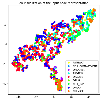
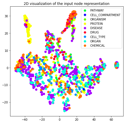
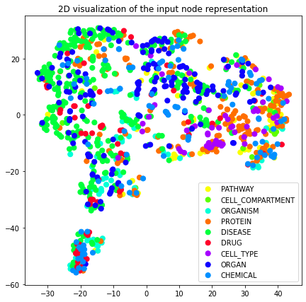
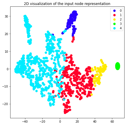
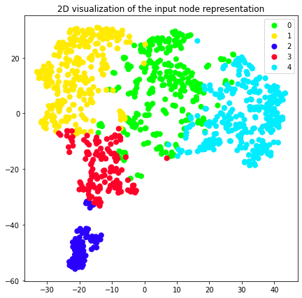
Plotting the embeddings
Having produced the embedding vectors, we can project them into a 2D space using dimensionality reduction techniques such as TSNE (t-distributed Stochastic Neighbor Embedding).
node2vec_2d = transform_to_2d(transformed_graph._nodes["node2vec"].tolist())
attri2vec_2d = transform_to_2d(transformed_graph._nodes["attri2vec"].tolist())
gcn_dgi_2d = transform_to_2d(transformed_graph._nodes["gcn_dgi"].tolist())
We can now plot these 2D vectors using the plot_2d util provided by
bluegraph.
plot_2d(transformed_graph, vectors=node2vec_2d, label_prop="entity_type")
plot_2d(transformed_graph, vectors=attri2vec_2d, label_prop="entity_type")
plot_2d(transformed_graph, vectors=gcn_dgi_2d, label_prop="entity_type")
Node similarity
We would like to be able to search for similar nodes using the computed
vector embeddings. For this we can use the NodeSimilarityProcessor
interfaces provided as a part of bluegraph.
We construct similarity processors for different embeddings and query
top 10 most similar nodes to the terms glucose and covid-19.
node2vec_l2 = NodeSimilarityProcessor(transformed_graph, "node2vec", similarity="euclidean")
node2vec_cosine = NodeSimilarityProcessor(
    transformed_graph, "node2vec", similarity="cosine")
node2vec_l2.get_neighbors(["glucose", "covid-19"], k=10)
{'glucose': {0.0: 'glucose',
  0.016042586: 'diabetic nephropathy',
  0.020855632: 'nonalcoholic fatty liver disease',
  0.020919867: 'hyperglycemia',
  0.027952814: 'metabolic syndrome',
  0.04255097: 'visceral',
  0.049424335: 'obesity',
  0.05932623: 'citrate',
  0.061201043: 'tissue factor',
  0.06682069: 'liver and intrahepatic bile duct disorder'},
 'covid-19': {0.0: 'covid-19',
  0.023866901: 'fatal',
  0.049039844: 'procalcitonin measurement',
  0.05976087: 'acute respiratory distress syndrome',
  0.08363058: 'neuromuscular',
  0.08448325: 'sterile',
  0.084664375: 'hydroxychloroquine',
  0.103314176: 'tidal volume',
  0.10976424: 'caspase-5',
  0.11111233: 'status epilepticus'}}
node2vec_cosine.get_neighbors(["glucose", "covid-19"], k=10)
{'glucose': {0.99999994: 'glucose',
  0.99718344: 'diabetic nephropathy',
  0.9968226: 'hyperglycemia',
  0.9958539: 'nonalcoholic fatty liver disease',
  0.9947761: 'metabolic syndrome',
  0.99151814: 'visceral',
  0.991088: 'respiration',
  0.9901221: 'obesity',
  0.9887427: 'liver and intrahepatic bile duct disorder',
  0.9885775: 'citrate'},
 'covid-19': {1.0: 'covid-19',
  0.99730766: 'fatal',
  0.9942852: 'procalcitonin measurement',
  0.9897085: 'acute respiratory distress syndrome',
  0.98890024: 'chronic obstructive pulmonary disease',
  0.9888062: 'sterile',
  0.98763454: 'neuromuscular',
  0.98537326: 'hydroxychloroquine',
  0.98534656: 'lopinavir/ritonavir',
  0.98470575: 'pulmonary'}}
attri2vec_l2 = NodeSimilarityProcessor(transformed_graph, "attri2vec")
attri2vec_cosine = NodeSimilarityProcessor(
    transformed_graph, "attri2vec", similarity="cosine")
attri2vec_l2.get_neighbors(["glucose", "covid-19"], k=10)
{'glucose': {0.0: 'glucose',
  0.0071316347: 'digestion',
  0.00823471: 'hepatocellular',
  0.0091231465: 'adipose tissue',
  0.010375342: 'axon',
  0.010453261: 'hemoglobin',
  0.010671802: 'bile',
  0.0106950635: 'vitamin',
  0.011250288: 'tissue',
  0.011955512: 'small intestine'},
 'covid-19': {0.0: 'covid-19',
  0.00061282323: 'chronic obstructive pulmonary disease',
  0.0009526084: 'vasculitis',
  0.0009802075: 'pulmonary edema',
  0.0010977304: 'liver failure',
  0.0011182561: 'inflammatory disorder',
  0.0011229385: 'parenteral',
  0.0012357396: 'osteoporosis',
  0.001249002: 'h1n1 influenza',
  0.0012659363: 'morphine'}}
attri2vec_cosine.get_neighbors(["glucose", "covid-19"], k=10)
{'glucose': {1.0: 'glucose',
  0.9778094: 'digestion',
  0.97610795: 'degradation',
  0.97395945: 'creatine',
  0.9727266: 'hepatocellular',
  0.9708393: 'adipose tissue',
  0.9704221: 'vitamin',
  0.9702778: 'astrocyte',
  0.9700098: 'hematopoietic stem cell',
  0.9698795: 'lymph node'},
 'covid-19': {1.0: 'covid-19',
  0.97816277: 'severe acute respiratory syndrome',
  0.9777578: 'middle east respiratory syndrome',
  0.9767103: 'respiratory failure',
  0.97613215: 'childhood-onset systemic lupus erythematosus',
  0.97379327: 'h1n1 influenza',
  0.9727: 'dengue fever',
  0.9719033: 'chronic obstructive pulmonary disease',
  0.97159684: 'arthritis',
  0.9704671: 'delirium'}}
gcn_l2 = NodeSimilarityProcessor(transformed_graph, "gcn_dgi")
gcn_cosine = NodeSimilarityProcessor(
    transformed_graph, "gcn_dgi", similarity="cosine")
gcn_l2.get_neighbors(["glucose", "covid-19"], k=10)
{'glucose': {0.0: 'glucose',
  0.0030039286: 'glucose tolerance test',
  0.0034940867: 'triglycerides',
  0.003617311: 'insulin',
  0.0036187829: 'high density lipoprotein',
  0.004899253: 'cholesterol',
  0.0056207227: 'organic phosphate',
  0.0057664528: 'uric acid',
  0.0058270395: 'fetus',
  0.006129055: 'diabetic nephropathy'},
 'covid-19': {0.0: 'covid-19',
  0.0009082245: 'coronavirus',
  0.002618216: 'fatal',
  0.0026699416: 'acute respiratory distress syndrome',
  0.0042233844: 'sars-cov-2',
  0.004636312: 'severe acute respiratory syndrome',
  0.004916654: 'middle east respiratory syndrome',
  0.005095474: 'myocarditis',
  0.0056914845: 'angiotensin ii receptor antagonist',
  0.0057702293: 'cardiac valve injury'}}
gcn_cosine.get_neighbors(["glucose", "covid-19"], k=10)
{'glucose': {1.0000001: 'glucose',
  0.98359084: 'triglycerides',
  0.9822164: 'cholesterol',
  0.981979: 'insulin',
  0.98167336: 'glucose tolerance test',
  0.979028: 'high density lipoprotein',
  0.9727696: 'low density lipoprotein',
  0.9723866: 'plasma',
  0.97019887: 'skeletal muscle tissue',
  0.9700538: 'atherosclerosis'},
 'covid-19': {0.99999994: 'covid-19',
  0.99609506: 'coronavirus',
  0.9897146: 'fatal',
  0.98897403: 'acute respiratory distress syndrome',
  0.98260605: 'sars-cov-2',
  0.980789: 'severe acute respiratory syndrome',
  0.9791904: 'middle east respiratory syndrome',
  0.97802055: 'myocarditis',
  0.97669864: 'angiotensin ii receptor antagonist',
  0.9753277: 'sars coronavirus'}}
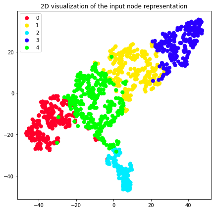
Node clustering
We can cluster nodes according to their node embeddings. Often such clustering helps to reveal the community structure encoded in the underlying networks.
In this example we will use the BayesianGaussianMixture model
provided by the scikit-learn to cluster the nodes according to different
embeddings into 5 clusters.
N = 5
X = transformed_graph.get_node_property_values("node2vec").to_list()
gmm = mixture.BayesianGaussianMixture(n_components=N, covariance_type='full').fit(X)
node2vec_clusters = gmm.predict(X)
X = transformed_graph.get_node_property_values("attri2vec").to_list()
gmm = mixture.BayesianGaussianMixture(n_components=5, covariance_type='full').fit(X)
attri2vec_clusters = gmm.predict(X)
X = transformed_graph.get_node_property_values("gcn_dgi").to_list()
gmm = mixture.BayesianGaussianMixture(n_components=5, covariance_type='full').fit(X)
gcn_dgi_clusters = gmm.predict(X)
Below we inspect the most frequent cluster members.
def show_top_members(clusters, N):
    for i in range(N):
        df = transformed_graph._nodes.iloc[np.where(clusters == i)]
        df.loc[:, "frequency"] = df.index.map(lambda x: graph._nodes.loc[x, "frequency"])
        print(f"#{i}: ", ", ".join(df.nlargest(10, columns=["frequency"]).index))
show_top_members(node2vec_clusters, N)
#0:  blood, heart, pulmonary, death, renal, hypertension, cardiovascular system, septicemia, oral cavity, fever
#1:  lung, survival, cancer, organ, plasma, angiotensin-converting enzyme 2, vascular, insulin, neutrophil, antibody
#2:  bacteria, antibiotic, pneumonia, escherichia coli, staphylococcus aureus, pathogen, klebsiella pneumoniae, microorganism, mucoid pseudomonas aeruginosa, organism
#3:  human, mouse, inflammation, animal, cytokine, interleukin-6, neoplasm, dna, tissue, proliferation
#4:  covid-19, infectious disorder, diabetes mellitus, sars-cov-2, liver, virus, brain, glucose, kidney, serum
/Users/oshurko/opt/anaconda3/envs/bg/lib/python3.7/site-packages/pandas/core/indexing.py:1667: SettingWithCopyWarning:
A value is trying to be set on a copy of a slice from a DataFrame.
Try using .loc[row_indexer,col_indexer] = value instead

See the caveats in the documentation: https://pandas.pydata.org/pandas-docs/stable/user_guide/indexing.html#returning-a-view-versus-a-copy
  self.obj[key] = value
show_top_members(attri2vec_clusters, N)
#0:  antibiotic, escherichia coli, staphylococcus aureus, klebsiella pneumoniae, mucoid pseudomonas aeruginosa, vancomycin, pseudomonas aeruginosa, ciprofloxacin, community-acquired pneumonia, staphylococcus
#1:  human, renal, survival, brain, hypertension, obesity, respiratory system, oral cavity, injury, oxygen
#2:  death, person, proliferation, molecule, lower, failure, intestinal, transfer, organism, sterile
#3:  dog, cat, water, depression, horse, anxiety, nasal, subarachnoid hemorrhage, proximal, brother
#4:  covid-19, blood, infectious disorder, heart, diabetes mellitus, lung, sars-cov-2, mouse, pulmonary, bacteria
show_top_members(gcn_dgi_clusters, N)
#0:  lung, sars-cov-2, liver, survival, virus, brain, glucose, kidney, cancer, serum
#1:  covid-19, blood, heart, diabetes mellitus, pulmonary, death, renal, hypertension, cardiovascular system, dog
#2:  bacteria, antibiotic, escherichia coli, staphylococcus aureus, pathogen, klebsiella pneumoniae, microorganism, mucoid pseudomonas aeruginosa, organism, sputum
#3:  infectious disorder, respiratory system, oral cavity, pneumonia, skin, fever, cystic fibrosis, urine, human immunodeficiency virus, influenza
#4:  human, mouse, inflammation, animal, cytokine, plasma, interleukin-6, insulin, neoplasm, dna
We can also use the previously plot_2d util and color our 2D nore
representation according to the clusters they belong to.
plot_2d(transformed_graph, vectors=node2vec_2d, labels=node2vec_clusters)
plot_2d(transformed_graph, vectors=attri2vec_2d, labels=attri2vec_clusters)
plot_2d(transformed_graph, vectors=gcn_dgi_2d, labels=gcn_dgi_clusters)
Node classification
Another downstream task that we would like to perform is node classification. We would like to automatically assign entity types according to their node embeddings. For this we will build predictive models for entity type prediction based on:
Only node features
Node2vec embeddings (only structure)
Attri2vec embeddings (structure and node features)
GCN Deep Graph Infomax embeddings (structure and node features)
First of all, we split the graph nodes into the train and the test sets.
train_nodes, test_nodes = model_selection.train_test_split(
    transformed_graph.nodes(), train_size=0.8)
Now we use the NodeClassifier interface to create our classification
models. As the base model we will use the linear SVM classifier
(LinearSVC) provided by scikit-learn.
features_classifier = NodeClassifier(LinearSVC(), feature_vector_prop="features")
features_classifier.fit(transformed_graph, train_elements=train_nodes, label_prop="entity_type")
features_pred = features_classifier.predict(transformed_graph, predict_elements=test_nodes)
node2vec_classifier = NodeClassifier(LinearSVC(), feature_vector_prop="node2vec")
node2vec_classifier.fit(transformed_graph, train_elements=train_nodes, label_prop="entity_type")
node2vec_pred = node2vec_classifier.predict(transformed_graph, predict_elements=test_nodes)
attri2vec_classifier = NodeClassifier(LinearSVC(), feature_vector_prop="attri2vec")
attri2vec_classifier.fit(transformed_graph, train_elements=train_nodes, label_prop="entity_type")
attri2vec_pred = attri2vec_classifier.predict(transformed_graph, predict_elements=test_nodes)
/Users/oshurko/opt/anaconda3/envs/bg/lib/python3.7/site-packages/sklearn/svm/_base.py:986: ConvergenceWarning: Liblinear failed to converge, increase the number of iterations.
  "the number of iterations.", ConvergenceWarning)
gcn_dgi_classifier = NodeClassifier(LinearSVC(), feature_vector_prop="gcn_dgi")
gcn_dgi_classifier.fit(transformed_graph, train_elements=train_nodes, label_prop="entity_type")
gcn_dgi_pred = gcn_dgi_classifier.predict(transformed_graph, predict_elements=test_nodes)
Let us have a look at the scores of different node classification models we have produced.
true_labels = transformed_graph._nodes.loc[test_nodes, "entity_type"]
get_classification_scores(true_labels, features_pred, multiclass=True)
{'accuracy': 0.59,
 'precision': 0.59,
 'recall': 0.59,
 'f1_score': 0.59,
 'roc_auc_score': 0.7847725250984877}
get_classification_scores(true_labels, node2vec_pred, multiclass=True)
{'accuracy': 0.36,
 'precision': 0.36,
 'recall': 0.36,
 'f1_score': 0.36,
 'roc_auc_score': 0.6786980556614562}
get_classification_scores(true_labels, attri2vec_pred, multiclass=True)
{'accuracy': 0.46,
 'precision': 0.46,
 'recall': 0.46,
 'f1_score': 0.46,
 'roc_auc_score': 0.7230397763375269}
get_classification_scores(true_labels, gcn_dgi_pred, multiclass=True)
{'accuracy': 0.33,
 'precision': 0.33,
 'recall': 0.33,
 'f1_score': 0.33,
 'roc_auc_score': 0.6585176007116533}
Link prediction
Finally, we would like to use the produced node embeddings to predict the existance of edges. This downstream task is formulated as follows: given a pair of nodes and their embedding vectors, is there an edge between these nodes?
As the first step of the edges prediciton task we will generate false edges for training (node pairs that don’t have edges between them).
false_edges = generate_negative_edges(transformed_graph)
We will now split both true and false edges into training and test sets.
true_train_edges, true_test_edges = model_selection.train_test_split(
    transformed_graph.edges(), train_size=0.8)
false_train_edges, false_test_edges = model_selection.train_test_split(
    false_edges, train_size=0.8)
And, finally, we will use the EdgePredictor interface to build our
model (using LinearSVC as before and the Hadamard product as the
binary operator between the embedding vectors for the source and the
target nodes.
model = EdgePredictor(LinearSVC(), feature_vector_prop="node2vec",
                      operator="hadamard", directed=False)
model.fit(transformed_graph, true_train_edges, negative_samples=false_train_edges)
true_labels = np.hstack([
    np.ones(len(true_test_edges)),
    np.zeros(len(false_test_edges))])
y_pred = model.predict(transformed_graph, true_test_edges + false_test_edges)
Let us have a look at the obtained scores.
get_classification_scores(true_labels, y_pred)
{'accuracy': 0.7333526166814736,
 'precision': 0.7333526166814736,
 'recall': 0.7333526166814736,
 'f1_score': 0.7333526166814736,
 'roc_auc_score': 0.6407728790685658}
Creating and saving embedding pipelines
bluegraph allows to create emebedding pipelines (using the
EmbeddingPipeline class) that represent a useful wrapper around a
sequence of steps necessary to produce embeddings and compute point
similarities. In the example below we create a pipeline for producing
attri2vec node embeddings and computing their cosine similarity.
We first create an encoder object that will be used in our pipeline as a preprocessing step.
definition_encoder = ScikitLearnPGEncoder(
    node_properties=["definition"], text_encoding_max_dimension=512)
We then create an embedder object.
D = 128
params = {
    "length": 5,
    "number_of_walks": 10,
    "epochs": 5,
    "embedding_dimension": D
}
attri2vec_embedder = StellarGraphNodeEmbedder(
    "attri2vec", feature_vector_prop="features", edge_weight="npmi", **params)
And finally we create a pipeline object. Note that in the code below we
use the SimilarityProcessor interface and not
NodeSimilarityProcessor, as we have done it previously. We use this
lower abstraction level interface, because the EmbeddingPipeline is
designed to work with any embedding models (not only node embedding
models).
attri2vec_pipeline = EmbeddingPipeline(
    preprocessor=definition_encoder,
    embedder=attri2vec_embedder,
    similarity_processor=SimilarityProcessor(
        FaissSimilarityIndex(
            similarity="cosine", dimension=D)))
We run the fitting process, which given the input data: 1. fits the encoder 2. transforms the data 3. fits the embedder 4. produces the embedding table 5. fits the similarity processor index
attri2vec_pipeline.run_fitting(graph)
link_classification: using 'ip' method to combine node embeddings into edge embeddings
How we can save our pipeline to the file system.
attri2vec_pipeline.save(
    "../data/attri2vec_test_model",
    compress=True)
And we can load the pipeline back into memory:
pipeline = EmbeddingPipeline.load(
    "../data/attri2vec_test_model.zip",
    embedder_interface=GraphElementEmbedder,
    embedder_ext="zip")
We can use retrieve_embeddings and get_similar_points methods of
the pipeline object to respectively get embedding vectors and top most
similar nodes for the input nodes.
pipeline.retrieve_embeddings(["covid-19", "glucose"])
[[0.07280001044273376,
  0.08163794130086899,
  0.08893375843763351,
  0.09304069727659225,
  0.11964225769042969,
  0.08136298507452011,
  0.0790518969297409,
  0.08503866195678711,
  0.08987397700548172,
  0.13234665989875793,
  0.06845631450414658,
  0.09433518350124359,
  0.057276081293821335,
  0.08183374255895615,
  0.0636567771434784,
  0.10424472391605377,
  0.06787201017141342,
  0.08923638612031937,
  0.07220311462879181,
  0.07509997487068176,
  0.09238457679748535,
  0.06531045585870743,
  0.0759056881070137,
  0.14457547664642334,
  0.08505883812904358,
  0.06661373376846313,
  0.07629712671041489,
  0.07443031668663025,
  0.07806529849767685,
  0.08416897058486938,
  0.12059333175420761,
  0.0758424922823906,
  0.10647209733724594,
  0.07496806234121323,
  0.09789688140153885,
  0.10009769350290298,
  0.09310337901115417,
  0.08175752311944962,
  0.08274300396442413,
  0.07131325453519821,
  0.12208940088748932,
  0.06224219128489494,
  0.09508002549409866,
  0.14279678463935852,
  0.057057347148656845,
  0.0588308647274971,
  0.08901730924844742,
  0.08926397562026978,
  0.0662379041314125,
  0.09682483226060867,
  0.07646792382001877,
  0.07486658543348312,
  0.070854052901268,
  0.054801177233457565,
  0.07894912362098694,
  0.060327619314193726,
  0.10469762980937958,
  0.07393162697553635,
  0.09346463531255722,
  0.09142538905143738,
  0.08995286375284195,
  0.057934362441301346,
  0.09345584362745285,
  0.09328961372375488,
  0.07854010164737701,
  0.07263723015785217,
  0.12583819031715393,
  0.06582190096378326,
  0.07038778066635132,
  0.06997384876012802,
  0.07740046083927155,
  0.0648268535733223,
  0.0915069580078125,
  0.1107659563422203,
  0.10443656146526337,
  0.06657622754573822,
  0.09377510845661163,
  0.06837121397256851,
  0.09725506603717804,
  0.060706377029418945,
  0.1157352551817894,
  0.0791042298078537,
  0.08426657319068909,
  0.06966130435466766,
  0.07881376147270203,
  0.06591648608446121,
  0.12842406332492828,
  0.09824175387620926,
  0.07571471482515335,
  0.0666264072060585,
  0.13996072113513947,
  0.10810025036334991,
  0.08261056989431381,
  0.062233999371528625,
  0.0959680825471878,
  0.0712309181690216,
  0.09311872720718384,
  0.08855060487985611,
  0.10211314260959625,
  0.0744297131896019,
  0.13628296554088593,
  0.07632824778556824,
  0.09952477365732193,
  0.09145186096429825,
  0.05990583822131157,
  0.08039164543151855,
  0.09073426574468613,
  0.0997760146856308,
  0.07251497358083725,
  0.06577309966087341,
  0.13079826533794403,
  0.08491260558366776,
  0.06395302712917328,
  0.04059096425771713,
  0.13386057317256927,
  0.07978139072656631,
  0.11739350110292435,
  0.05938231945037842,
  0.09113242477178574,
  0.04842013493180275,
  0.05951233580708504,
  0.0531817302107811,
  0.07620435208082199,
  0.0648634135723114,
  0.07864787429571152,
  0.16829492151737213,
  0.08553200215101242,
  0.10460848361253738],
 [0.10236917436122894,
  0.09674006700515747,
  0.07649692893028259,
  0.0845288410782814,
  0.0760805606842041,
  0.09261447936296463,
  0.09488159418106079,
  0.12473700195550919,
  0.0718981921672821,
  0.1021432876586914,
  0.09268027544021606,
  0.09814798831939697,
  0.09521770477294922,
  0.10098892450332642,
  0.09244446456432343,
  0.0635334774851799,
  0.09584149718284607,
  0.08556737005710602,
  0.0852125957608223,
  0.07645734399557114,
  0.08095100522041321,
  0.09593727439641953,
  0.08347492665052414,
  0.08885250240564346,
  0.08701310306787491,
  0.09694880247116089,
  0.11121281236410141,
  0.08294625580310822,
  0.08726843446493149,
  0.0701715424656868,
  0.09523919224739075,
  0.07785829901695251,
  0.09603790938854218,
  0.0824458971619606,
  0.08737047761678696,
  0.08853974938392639,
  0.06570149958133698,
  0.10123683512210846,
  0.07348940521478653,
  0.06943066418170929,
  0.1299903839826584,
  0.08817175030708313,
  0.06109187752008438,
  0.08437755703926086,
  0.08351798355579376,
  0.08457473665475845,
  0.07322832942008972,
  0.09192510694265366,
  0.08886606246232986,
  0.07747369259595871,
  0.07242843508720398,
  0.09057212620973587,
  0.10816606134176254,
  0.09043016284704208,
  0.09076884388923645,
  0.09677130728960037,
  0.08017739653587341,
  0.10074104368686676,
  0.07700169831514359,
  0.07268036901950836,
  0.07325926423072815,
  0.07274069637060165,
  0.06991708278656006,
  0.0845450609922409,
  0.06915223598480225,
  0.0702526643872261,
  0.09593337029218674,
  0.09438585489988327,
  0.08171636611223221,
  0.07945361733436584,
  0.0642147958278656,
  0.08085450530052185,
  0.0607246495783329,
  0.08492715656757355,
  0.07719805836677551,
  0.10578399896621704,
  0.10591499507427216,
  0.09201952069997787,
  0.0818672627210617,
  0.08240731060504913,
  0.06790471076965332,
  0.07807260751724243,
  0.0730040892958641,
  0.1071859821677208,
  0.11890396475791931,
  0.056871384382247925,
  0.09596915543079376,
  0.07900075614452362,
  0.09519974142313004,
  0.10644269734621048,
  0.08464374393224716,
  0.10578206926584244,
  0.10132604092359543,
  0.07531124353408813,
  0.09358139336109161,
  0.07341431826353073,
  0.09914236515760422,
  0.07994917780160904,
  0.06680438667535782,
  0.07904554903507233,
  0.09318091720342636,
  0.08036279678344727,
  0.07590607553720474,
  0.07815994322299957,
  0.10222751647233963,
  0.11459968239068985,
  0.0987963154911995,
  0.08063937723636627,
  0.10191671550273895,
  0.11327352374792099,
  0.08440998196601868,
  0.09114128351211548,
  0.0879993736743927,
  0.0869138091802597,
  0.1110539585351944,
  0.08841552585363388,
  0.08597182482481003,
  0.09037397056818008,
  0.07773328572511673,
  0.09250291436910629,
  0.09562606364488602,
  0.07948072999715805,
  0.08507171273231506,
  0.08046958595514297,
  0.08189624547958374,
  0.07476285845041275,
  0.10559207946062088,
  0.10403718799352646]]
a = pipeline.retrieve_embeddings(["covid-19", "glucose"])
pipeline.get_neighbors(existing_points=["covid-19", "glucose"], k=5)
([array([1.0000001 , 0.98876834, 0.9861363 , 0.9855296 , 0.98494315],
        dtype=float32),
  array([1.0000001 , 0.98885393, 0.98832536, 0.9882704 , 0.9882704 ],
        dtype=float32)],
 [Index(['covid-19', 'middle east respiratory syndrome',
         'severe acute respiratory syndrome',
         'childhood-onset systemic lupus erythematosus', 'h1n1 influenza'],
        dtype='object', name='@id'),
  Index(['glucose', 'fatigue', 'anorexia', 'congenital abnormality', 'proximal'], dtype='object', name='@id')])